Cohort-by-time effect matrices and heatmaps

library(nonabsdid)

This is a separate feature line from the event-study workflow in Getting started. It supports DCDH and the fect family only; see Why not PanelMatch? below.

Event study vs. effect matrix

The main nonabsdid workflow ([nabs_event_study()] / [nabs_event_plot()]) collapses every treated cohort onto a single relative-time axis: one curve per estimator. That is the right summary most of the time, but it hides which cohorts drive the average.

The effect matrix keeps the onset cohort as a second dimension. Instead of a curve you get a grid – rows are onset cohorts, columns are relative (or calendar) time, and the fill is the estimated effect – drawn as a heatmap. It is the two-dimensional companion to the event-study overlay, built from the same estimator objects.

Three user-facing pieces mirror the event-study API:

nabs_effect_cells() – fit one estimator and return its cohort cells.
as_nabs_effect_cells() – coerce an existing estimator object into the cell schema.
plot_effect_matrix() – draw one or more cell tables as heatmaps.

A toy non-absorbing panel

set.seed(1)
N <- 120; TT <- 14
panel <- expand.grid(id = 1:N, t = 1:TT)
grp   <- panel$id %% 4                         # group 0 = never treated
onset <- c(`1` = 4L, `2` = 6L, `3` = 8L)[as.character(grp)]
# a quarter of switchers turn OFF again 3 periods later (non-absorbing)
off   <- (panel$id %% 8 == 1) & !is.na(onset) & panel$t >= onset + 3L
panel$d <- as.integer(!is.na(onset) & panel$t >= onset & !off)
panel$y <- rnorm(N, sd = .5)[panel$id] + 0.15 * panel$t +
  ifelse(panel$d == 1, 0.4, 0) + rnorm(nrow(panel))

One-step fit: `nabs_effect_cells()`

nabs_effect_cells() wires up what a cohort breakdown needs for each estimator (a unit-level onset cohort for DCDH; keep.sims = TRUE for fect bootstrap cell SEs), so you only pass the usual arguments.

res_ife <- nabs_effect_cells(
  panel, outcome = "y", treatment = "d", unit = "id", time = "t",
  method = "IFE", lags = 4, leads = 6, nboots = 100
)
#> For identification purposes, units whose number of untreated periods <5 are dropped automatically.
#> Cross-validating ...
#> Criterion: Mean Squared Prediction Error
#> Interactive fixed effects model...
#> r = 2; sigma2 = 0.89113; IC = 2.40771; PC = 2.98096; MSPE = 2.70052
#> 
#>  r* = 2
res_ife$cells
#> # <nabs_effect_cell_tbl>: 19 cells, 3 cohorts, methods: "IFE"
#> # A tibble: 19 × 12
#>    cohort event_time calendar_time estimate std.error conf.low conf.high     n
#>     <int>      <int>         <int>    <dbl>     <dbl>    <dbl>     <dbl> <int>
#>  1      4          0             4  0.938       0.700   -0.848     0.903    15
#>  2      4          1             5  0.580       0.672   -1.91      1.30     15
#>  3      4          2             6  1.06        0.889   -1.34      1.45     15
#>  4      6          0             6  0.260       0.477   -0.801     1.07     30
#>  5      6          1             7  0.388       0.346   -0.771     0.757    30
#>  6      6          2             8  0.0478      0.643   -0.939     1.96     30
#>  7      6          3             9  0.667       0.679   -0.736     2.20     30
#>  8      6          4            10  1.29        1.00    -1.31      2.48     30
#>  9      6          5            11  0.921       0.735   -1.10      1.92     30
#> 10      6          6            12  0.682       0.611   -0.769     1.95     30
#> 11      6          7            13  0.130       0.648   -1.45      0.906    30
#> 12      6          8            14 -0.0850      0.684   -1.08      1.69     30
#> 13      8          0             8  0.278       0.637   -1.17      1.31     30
#> 14      8          1             9  0.680       0.677   -1.10      1.48     30
#> 15      8          2            10  0.800       1.13    -2.69      2.43     30
#> 16      8          3            11  0.778       0.716   -1.15      1.55     30
#> 17      8          4            12  0.655       0.513   -0.431     1.74     30
#> 18      8          5            13 -0.00298     0.800   -1.04      1.17     30
#> 19      8          6            14 -0.280       0.809   -0.901     1.85     30
#> # ℹ 4 more variables: window <chr>, method <chr>, outcome <chr>,
#> #   se_method <chr>

plot_effect_matrix(res_ife$cells, show_estimates = TRUE, show_se = TRUE)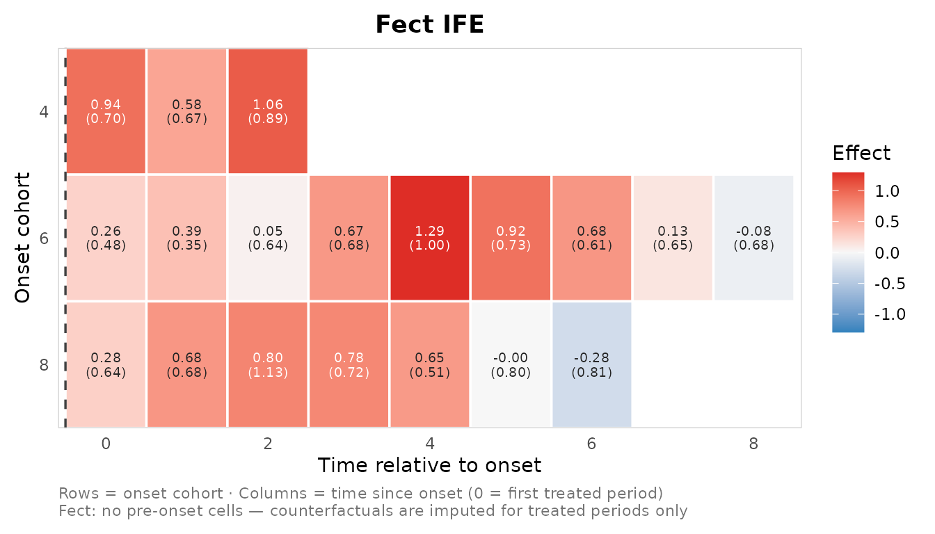

A single-method call is titled with the method automatically, and show_se = TRUE prints the standard error (in parentheses) beneath each estimate. The fect surface only covers treated cells, so the matrix starts at event_time = 0 (the first treated period) and has no pre-period column.

For DCDH, dcdh_strategy = "loop" (the default) re-estimates the event study once per onset cohort against the never-treated units; "by" instead issues a single did_multiplegt_dyn(..., by = cohort) call.

res_dcdh <- nabs_effect_cells(
  panel, outcome = "y", treatment = "d", unit = "id", time = "t",
  method = "DCDH", lags = 3, leads = 5, dcdh_strategy = "loop"
)
#> ℹ Attached polars for the DCDH backend.
#> The number of placebos which can be estimated is at most 2.The command will therefore try to estimate 2 placebo(s).

plot_effect_matrix(res_dcdh$cells, show_estimates = TRUE, show_se = TRUE)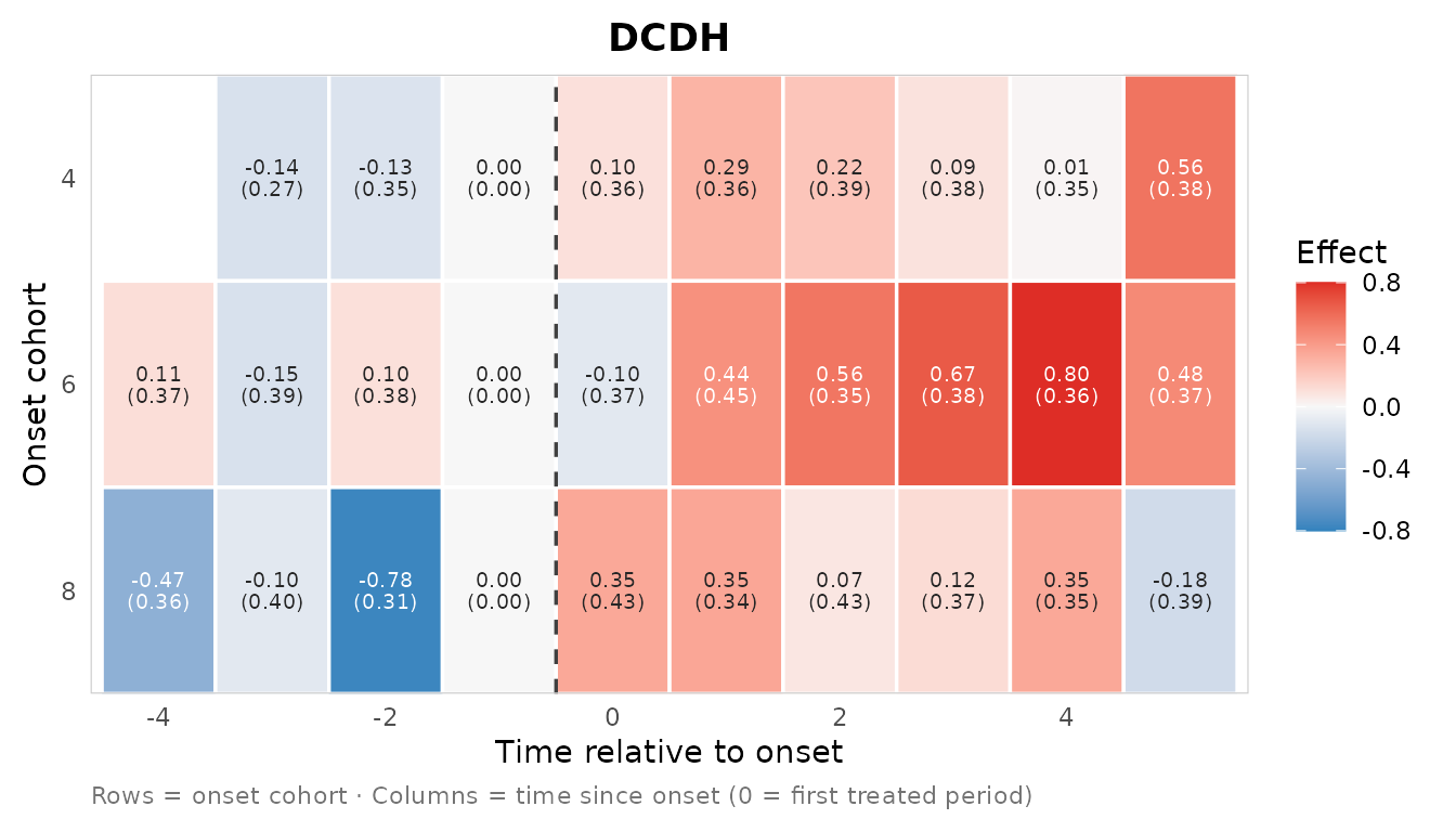

Unlike fect, DCDH reports placebo (pre-period) cells and a reference period (normalized to 0 at event_time = -1), so its matrix spans negative event time too.

Comparing methods

The recommended view is one heatmap per method (above): each is titled with its method and stays readable. If you do want them in one figure, passing several cell tables facets them with a shared fill scale and legend:

plot_effect_matrix(res_dcdh$cells, res_ife$cells)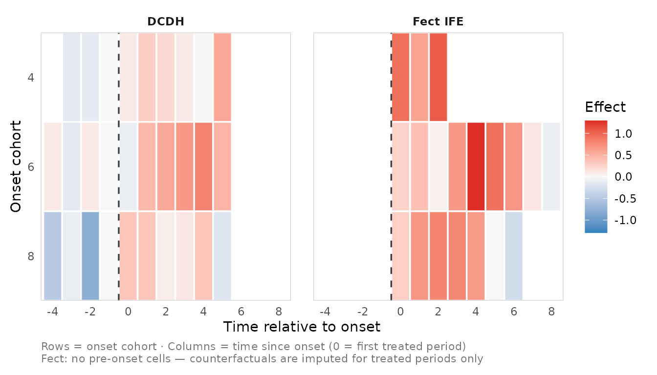

The faceted view is convenient but gets crowded fast (especially with in-tile labels), which is why per-method plots are the default emphasis.

Either way, read this as triangulation of the pattern, not as cell-by-cell equality. The two estimators line up on the same axes – both define the cohort as the onset period and anchor event_time = 0 at the first treated period – but they do not target identical quantities:

Different estimands / identification. fect imputes a counterfactual ( $Y - \hat Y(0)$ ) from a fixed-effects / factor model; DCDH forms long differences from the period before each switch. Level offsets between the two are expected.
Different controls. The DCDH "loop" strategy compares each cohort to the never-treated; fect’s counterfactual is model-based over all controls.
Different coverage. fect is post-only; DCDH adds placebos and a reference cell.
Non-absorbing wrinkle. The cohort is the first onset. Units that switch off and on again contribute to large-event_time cells under both methods, but each handles carryover differently, so those cells are the least comparable.

The fill encodes the point estimate only. Standard errors live in the std.error column and can be drawn in each tile with show_se = TRUE ("bootstrap" for fect, "native" or CI-recovered "ci" for DCDH; see the schema below). For claims about whether two cells differ, look at those SEs rather than the colours.

Working from existing objects

If you already fit an estimator, coerce it with as_nabs_effect_cells(). For fect you need imputed_outcomes() (fect >= 2.4.0); for bootstrap cell SEs the fit must have been run with se = TRUE, keep.sims = TRUE. For DCDH, pass an object run with a unit-level cohort by variable.

fit <- fect::fect(y ~ d, data = panel, index = c("id", "t"),
                  method = "fe", force = "two-way",
                  se = TRUE, nboots = 100, keep.sims = TRUE)
cells <- as_nabs_effect_cells(fit, method = "FE", outcome = "y")

A data-frame escape hatch needs no estimator packages – handy for testing the plot or building cells from numbers you already have:

raw <- expand.grid(cohort = c(4L, 6L, 8L), event_time = -2:5)
raw$estimate  <- with(raw, ifelse(event_time < 0, 0, 0.4 + 0.05 * event_time))
raw$std.error <- 0.07
cells <- as_nabs_effect_cells(raw, method = "FE", outcome = "y")
plot_effect_matrix(cells, show_estimates = TRUE, show_se = TRUE)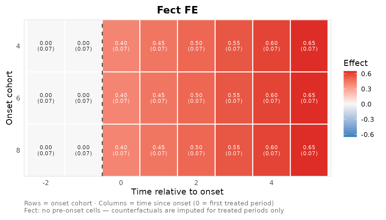

Collapsing back to an event study

aggregate_effects() averages cells over cohorts and returns a nabs_event_study_tbl, making explicit that the event study is the cohort-collapsed view of the same cells. (Re-aggregated standard errors are not computed, so they come back NA; use it for a quick overlay, not inference.)

agg <- aggregate_effects(res_ife$cells, by = "event_time")
#> ℹ Aggregated over cohorts; std.error is "NA" (re-aggregated SEs need replicate
#>   draws).
nabs_event_plot(agg, xlim = c(0, 6))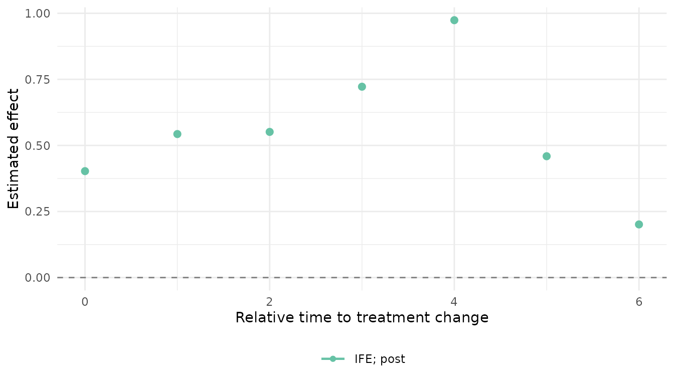

The cell schema

as_nabs_effect_cells() returns a tibble of class nabs_effect_cell_tbl:

column	type	description
`cohort`	int	Onset calendar period (first treated period).
`event_time`	int	Relative period; `0` = onset.
`calendar_time`	int	`cohort + event_time` (may be `NA`).
`estimate`	num	Cell point estimate.
`std.error`	num	Standard error (may be `NA`).
`conf.low/high`	num	CI bounds.
`n`	int	Treated cells aggregated (fect only; `NA` for DCDH).
`window`	chr	`"pre"` / `"post"`.
`method`	chr	Estimator label.
`outcome`	chr	Outcome name.
`se_method`	chr	`"bootstrap"` (fect), `"native"`/`"ci"` (DCDH), or `"none"`.

The se_method column records how uncertainty was produced. fect cells use the bootstrap surface (imputed_outcomes(replicates = TRUE)), re-aggregated within each replicate; DCDH cells carry the estimator’s own SEs; otherwise SEs are NA.

Why not PanelMatch?

A faithful cohort matrix needs cohort-level estimates and cohort-level uncertainty. For DCDH and fect both fall out of objects the packages already expose. PanelMatch reports lead-specific ATTs aggregated over all matched sets; recovering a per-cohort cell means re-aggregating matched-set effects by switch time and re-running the matched-set bootstrap on that re-aggregation to get honest SEs. That is real work and out of scope for this pass, so PanelMatch is omitted here rather than shipped with naive (wrong) standard errors. The se_method column is reserved so a PanelMatch path can slot in later without changing the plotting code.