Base-R surface views of a TROP penalty-sensitivity grid

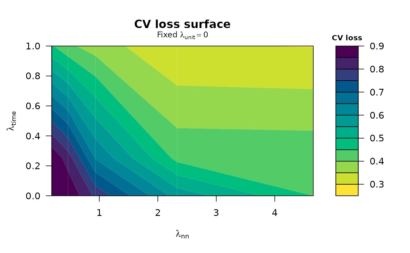
Draws the cross-validation-loss surface and the ATT surface from a trop_sensitivity() grid as two separate, full-width base-graphics plots, each with a colour key (legend) on the right. Unlike autoplot.cf_trop_grid() — a single ggplot2 heatmap that packs both into one panel — this view keeps the surfaces apart so neither is squeezed, and needs no ggplot2. The surface axes follow the swept penalties recorded on the grid (see the axes argument of trop_sensitivity()).

Usage

plot_trop_surfaces(
  grid,
  which = c("both", "cv_loss", "att"),
  ask = interactive(),
  ...
)

Arguments

grid

A cf_trop_grid returned by trop_sensitivity().

which

Which surface(s) to draw: "both" (default), "cv_loss", or "att". With "both" the two surfaces are drawn as separate figures; on an interactive screen device you are prompted between them (use a multi-page device such as pdf(), or call once per surface, to keep both).

ask

Logical; when drawing both on an interactive device, prompt before the second figure. Defaults to interactive().

...

Further arguments passed to graphics::filled.contour().

Value

Invisibly, a list with the cv_loss and att surface matrices (rows = y-axis penalty, columns = x-axis penalty).

See also

trop_sensitivity(), autoplot.cf_trop_grid()

Examples

# \donttest{
df <- sim_panel(N = 14, T = 9, n_treated = 3, t0 = 6, att = 2, seed = 1)
g <- trop_sensitivity(df, "y", "w", "id", "t",
                      lambda_time = c(0, 0.25, 1),
                      control = trop_control(n_cv_cells = 5L, cv_cycles = 1L,
                                             tol = 1e-3, seed = 1L))
plot_trop_surfaces(g, which = "cv_loss")

# }