TROP penalty-sensitivity grid (heatmap data)

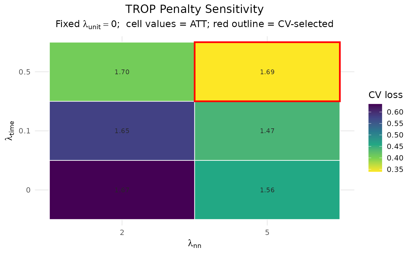
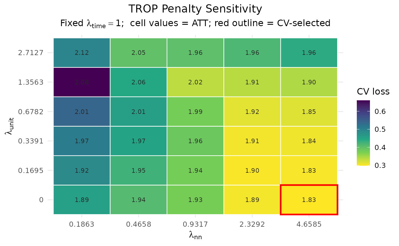
Sweeps any two of the three TROP penalties — \(\lambda_{time}\), \(\lambda_{unit}\) and \(\lambda_{nn}\) — against each other while holding the third fixed, and records at each grid point both the resulting ATT estimate and the leave-one-out cross-validation loss. This is the data behind the diagnostic heatmap: colour the cells by CV loss to see where the data-driven choice lands, and read the ATT off each cell to judge how sensitive the estimate is to the penalties. Use axes to choose which two penalties go on the x and y axes; the remaining (fixed) penalty is reported in the heatmap subtitle.

Usage

trop_sensitivity(
  data,
  outcome,
  treatment,
  unit,
  time,
  lambda_time = NULL,
  lambda_nn = NULL,
  lambda_unit = NULL,
  axes = c("nn", "time"),
  anchor = "pooled",
  control = trop_control(),
  seed = NULL,
  verbose = FALSE
)

Arguments

data

A long data.frame, one row per unit-time.

outcome, treatment, unit, time

Column names (strings).

lambda_time, lambda_nn, lambda_unit

Penalty inputs. For a penalty that is on an axis (see axes), supply a numeric grid to sweep (or NULL for a data-driven default grid; the lambda_nn default keeps only the finite part, as the heatmap axis needs finite values). For the penalty held fixed, supply a single value, or NULL to choose it once by cross-validation and hold it fixed across the sweep.

axes

Length-2 character vector naming the two penalties to sweep, as c(x, y): the first is the x axis, the second the y axis. Each must be one of "time", "unit", "nn". Defaults to c("nn", "time") (the historical layout). The third penalty is held fixed.

anchor

Estimation anchor passed to the ATT computation ("pooled" by default for speed).

control

A list of solver/CV controls from trop_control().

seed

Optional integer seed for CV-cell sampling.

verbose

Logical; print progress.

Value

A cf_trop_grid (a data.frame) with columns lambda_time, lambda_nn, lambda_unit, att, cv_loss. The two swept penalties vary across rows; the fixed penalty is constant. The grid point minimising cv_loss (the data-driven choice) is stored in attr(., "selected"), and the chosen layout in attr(., "axes") (named x/y) and attr(., "fixed").

See also

trop(), autoplot.cf_trop_grid()

Examples

# \donttest{
df <- sim_panel(N = 14, T = 9, n_treated = 3, t0 = 6, att = 2, seed = 1)
g <- trop_sensitivity(df, "y", "w", "id", "t",
                      lambda_time = c(0, 0.1, 0.5), lambda_nn = c(2, 5),
                      control = trop_control(n_cv_cells = 5L, cv_cycles = 1L,
                                             tol = 1e-3, seed = 1L))
autoplot(g)


# Sweep the unit penalty against the nuclear-norm penalty instead, holding
# the time penalty fixed (chosen by CV):
g2 <- trop_sensitivity(df, "y", "w", "id", "t", axes = c("nn", "unit"),
                       control = trop_control(n_cv_cells = 5L, cv_cycles = 1L,
                                              tol = 1e-3, seed = 1L))
autoplot(g2)

# }