Estimation-RMSE curve over one design dimension

Sweeps one design dimension – the number of control units ("n_control"), pre-treatment periods ("n_pre"), treated units ("n_treated") or post-treatment periods ("n_post") – and, at each value, runs a semi-synthetic Monte Carlo: panels are drawn from a latent factor model in which treatment is selected on the factor loadings (so plain DID/TWFE is biased), a known constant effect att is imposed, every estimator is run, and the estimation RMSE against the known truth is recorded. 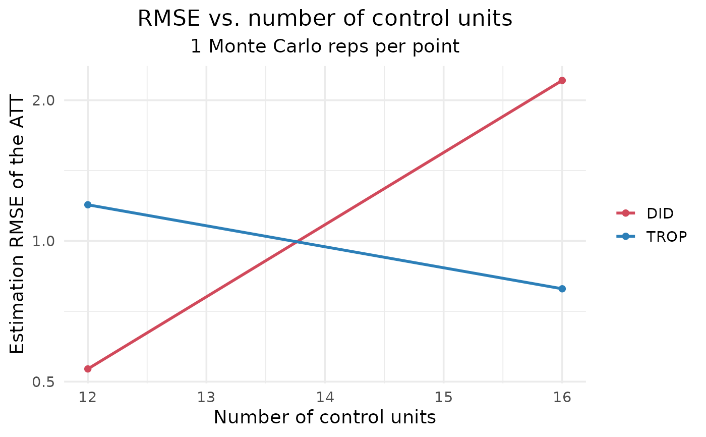The result is the data behind the paper-style "RMSE vs. N_control / T_pre" line plot, one line per estimator. With a dense values grid and enough n_runs the curves are smooth, as in the paper.

Usage

rmse_curve(
  vary = c("n_control", "n_pre", "n_treated", "n_post"),
  values = NULL,
  n_runs = 500L,
  methods = c("DID", "SDID", "SC", "MC", "DIFP", "TROP"),
  exclude = NULL,
  n_control = 60L,
  n_treated = 8L,
  n_pre = 16L,
  n_post = 6L,
  rank = 4L,
  att = 2,
  noise = 1,
  ar = 0.4,
  trend_sd = 0.05,
  anchor = "pooled",
  control = trop_control(),
  seed = 1L,
  parallel = FALSE,
  progress = interactive(),
  verbose = FALSE
)

Arguments

vary: Which dimension to sweep: "n_control", "n_pre", "n_treated" or "n_post".
values: Integer vector of values for the swept dimension. Defaults to seq(20, 45, by = 5) for control units, seq(5, 38, by = 2) for pre-periods, and seq(2, 12, by = 2) for treated units or post-periods. Each value is an actual measured point (its own Monte Carlo); pass a denser/wider grid for smoother or longer curves.
n_runs: Monte Carlo replications per value (higher = smoother; the paper uses ~1000). Default 500. Note: with the dense default grid and six estimators this is a large simulation (thousands of fits per panel); reduce n_runs and/or values for a quick look, or parallelise the outer loop.
methods: Estimators to include; any subset of the panel_compare() methods. Default c("DID", "SDID", "SC", "MC", "DIFP", "TROP"), the six estimators compared in the paper. gsynth, augsynth and CS can be added if those packages are installed.
exclude: Optional character vector of methods to drop from methods (e.g. exclude = "DIFP"). Unknown names are ignored with a warning.
n_control, n_treated, n_pre, n_post: Base design; the dimension named in vary is overridden by values, the rest are held fixed. Defaults give a sizeable panel (60 controls, 8 treated, 16 pre- and 6 post-periods).
rank, att, noise: Number of latent factors, the imposed (true) ATT, and the idiosyncratic-noise scale.
ar: AR(1) coefficient of the idiosyncratic errors (serial correlation).
trend_sd: SD of the heterogeneous unit-specific linear trend slopes (non-parallel trends); treatment is also selected on this slope.
anchor: Estimation anchor for the native ATT ("pooled" by default for speed across the many fits).
control: Solver/CV controls from trop_control().
seed: Base integer seed (each replication uses a distinct offset).
parallel: Logical; if TRUE and the future.apply package is installed, the Monte Carlo tasks are run in parallel honouring the active future plan (e.g. future::plan(future::multisession, workers = 6)). Results are identical to the sequential default because each task is self-seeded. Default FALSE.
progress: Logical; print a rough progress indicator (completed fits, a percentage, elapsed time and an ETA) periodically while the curve runs. Helpful for the heavy large-n_runs jobs. Defaults to interactive(), so it shows in an interactive session and stays silent in scripts and tests. Messages go to stderr(); wrap in suppressMessages() to mute.
verbose: Logical; additionally print a line as each swept value finishes. Independent of progress.

Value

A cf_rmse_curve (a data.frame) with columns method, x (the swept value), rmse, bias, n_runs. The swept-dimension label is in attr(., "vary").

Details

This is a simulation diagnostic on synthetic data; it does not take a user panel. To run a curve on your own data, draw panels with sim_semisynthetic() and call panel_compare() in a loop.

Examples

# \donttest{
# quick look (small grid + few reps); raise n_runs/values for paper quality
cc <- rmse_curve("n_control", values = c(12, 16), n_runs = 1, n_pre = 6, n_post = 3,
                 n_treated = 2, methods = c("DID", "TROP"),
                 control = trop_control(n_cv_cells = 5L, cv_cycles = 1L,
                                        tol = 1e-3, seed = 1L))
autoplot(cc)

# }