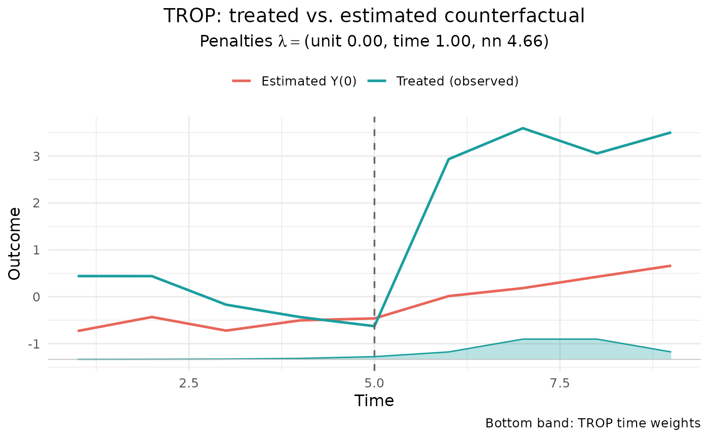
Synthetic-control-style trajectory plot for a single TROP fit

Draws the treated-unit average observed path against the estimated untreated (counterfactual) path, in the style of the synthdid plot: a dashed line marks the last pre-treatment period, the post-treatment gap between the two lines is the estimated effect, and – since TROP carries explicit time weights – the time weights \(\theta_s = \exp(-\lambda_{time} |t - s|)\) are drawn as a filled band along the bottom (as in synthdid's time-weight strip) to show which periods the counterfactual leans on. The band shows weights, not observation counts; heights are scaled to the largest weight, and with \(\lambda_{time} = 0\) the weights are uniform and the band is flat.

Usage

# S3 method for class 'trop'
autoplot(object, show_weights = TRUE, show_se = FALSE, ...)

Arguments

object: A trop fit from trop().
show_weights: Logical; draw the time-weight band along the bottom.
show_se: Logical; append the fit's standard-error method to the subtitle. Defaults to FALSE because this plot does not display standard errors – see trop_event_study() for the uncertainty visualisation.
...: Unused.

Value

A ggplot object.

Details

This is a point-estimate trajectory: it shows no standard errors or confidence intervals (the post-treatment gap is left unshaded so it is not mistaken for a confidence band). To visualise the fit's uncertainty, use trop_event_study() and call autoplot() on the result, which draws per-period estimates with pointwise confidence bars. Accordingly the subtitle reports only the selected penalties by default; set show_se = TRUE to also note which standard-error method the fit used.

Examples

# \donttest{
df <- sim_panel(N = 14, T = 9, n_treated = 3, t0 = 6, att = 3, seed = 1)
autoplot(trop(df, "y", "w", "id", "t", se = "none",
              control = trop_control(n_cv_cells = 5L, cv_cycles = 1L,
                                     tol = 1e-3, seed = 1L)))

# }